Data handling and visualization using Python
CNRCWP: student workshop
Oleksandr (Sasha) Huziy
UQÀM, December 2013
 |
Outline part I
Python basics
Builtin data types
Operations on file system, strings and dates
Modules, classes and functions
Libraries for scientific computing
- NumPy/SciPy
Handling NetCDF4 files
- Netcdf4-python
Introduction and history
Python is an interpreted, strictly typed programming language developed by Guido Van Rossum.
It was created in 90s of the previous century and has seen 3 major releases from that time.
There many implementations of Python (in C, Java, Python, ...), CPython implementation is used most widely and we are going to use it during the tutorial.
Talk on Python history by Guido Van Rossum here.
Syntax
#Variable decalaration <-This is a comment
a = 10; b = "mama"; x = None;

x = [1,2,4, 5, "I am a fifth element"]
#looping
for el in x:
    #Checking conditions
    if isinstance(el, int):
        print(el ** 2 % 10),
    else:
        msg = ", but my index is {0}."
        msg = msg.format(x.index(el))
        print(el + msg),

#now we are outside of the loop since no identation
print "\nSomething ..."
Syntax
#accessing elements of a list
x[3], x[-1], x[1:-1]
Defining functions
def myfirst_func(x, name = "Sasha"):
    """
    This is the comment describing method
    arguments and what it actually does
    x - dummy argument that demonstrates
    use of positional arguments
    name - demonstrates use of keyword arguments
    """
    print "Hello {0} !!!".format(name)
    return 2, None, x
Calling functions
#Calling the function f
myfirst_func("anything", name = "Oleks")
Defining a class
from datetime import datetime

class Person(object):
    #Example of a static class variable
    population = 0
    def __init__(self, name = "Sasha"):
        Person.population += 1
        #instance fields
        self._birthdate = datetime.now() #private attribute (conv.)
        self.name = name #public attribute

    def my_moto(self):
        return "Go go {0}!!!".format(self.name)

    def get_my_age(self):
        return datetime.now() - self._birthdate
Creating and manipulating objects
p1 = Person() #Creating an object of class Person
##Create some more person objects
for i in range(10):
    p = Person(name = str(i))

import time
time.sleep(5) #wait for 5 seconds
print p.my_moto()
print "{0} persons were born.".format(p1.population)
print "The age of the first is {0}".format(p1.get_my_age())
Python basics - code hierarchy
Each python file is a python module, it can contain function and class definitions
A folder with python files and a file
__init__.py(might be empty file) is called package
Exercises on basic syntax
Create a script
hello.pyin your favourite editor and addprint "Hello world", save and run it:python hello.pyModify the script making it print squares of odd numbers from 13 to 61 inclusively.
What will this code print to console:
    x = 1 #define a global variable
    def my_function(argument = x):
        print argument ** 2
    #change the value of the global variable
    x = 5
    my_function() #call the function defined above
Builtin data containers
Python provides the following data structures. Which are actually classes with attributes and methods.
list(range, *, +, pop, len, accessing list elements, slices, last element, 5 last elements)tuple(not mutable, methods)dict(accessing elements, keys, size)set(set theoretical operations, cannot have 2 equal elements)
Builtin data containers (lists)
#lists (you can conactenate and sort in place)
the_list = [1,2,3,4,5]; other_list = 5 * [6];
print the_list + other_list
#Test if a number is inside a list
print 19 in the_list, 5 in the_list, (6 in the_list and 6 in other_list)
Builtin data containers (lists)
#square eleaments of a list
#list comprehension
print [the_el ** 2 for the_el in the_list]
#Generating list or iterable of integers
print range(1,20)
Builtin data containers (lists)
##There are some utility functions that can be applied to lists
print sum(the_list), \
      reduce(lambda x, y: x + y, the_list)
#loop through several lists at the same time
for el1, el2 in zip(the_list, other_list):
    print(el1+el2),
Builtin data containers (tuples)
the_tuple = (1,2,3) #tuple is an immutable list, is hashable
print the_tuple[-1]
Builtin data containers (tuples)
#tuples are immutable, e.g:
try:
    the_tuple[1] = 25
except TypeError, te:
    print te
Builtin data containers (dictionary)
#dictionary
author_to_books = {
"Stephen King":
    ["Carrie","On writing","Green Mile"],

"Richard Feynman":
    ["Lectures on computation",
     "The pleasure of finding things out"]
}
#add elements to a dictionary
author_to_books["Andrey Kolmogorov"] = \
        ["Foundations Of The Theory Of Prob..."]
Builtin data containers (dictionary)
#print the list of authors
print author_to_books.keys()
#Iterate over keys and values
for author, book_list in author_to_books.iteritems():
    suffix = "s" if len(book_list) > 1 else ""
    print("{0} book{1} by {2};\n".format(len(book_list), suffix, author)),
Exercises: builtin containers
Find a sum of squares of all odd integers that are smaller than 100 in one line of code (Hint: use list comprehensions)
Find out what does
enumeratedo.Implement recursive fibonacci function with caching, which given the index of a fibonacci number returns its value.
Modules and classes to operate on
File system (
os, shutil, sys)- create folder, list folder contents, check if file or folder exists
Strings (+, *, join, split, regular expressions)
Dates (datetime, timedelta, )
File system
import os
#print current directory
print os.getcwd()
File system
#get list of files in the current directory
flist = os.listdir(".")
print flist[:7]
File system
#Check if file exists
fname = flist[0]
print fname,":", os.path.isfile(fname), \
      os.path.isdir(fname),  \
      os.path.islink(fname)
You might also find useful the following modules: sys, shutil, path
Strings
s = "mama"
#reverse (also works for lists)
print s[-1::-1]
#Dynamically changing parts of a string
tpl = "My name is {0}. I am doing my {1}.\nI am {2} old.\nWeight is {3:.3f} kg"
print tpl.format("Black", "PhD", 25, 80.7823)
Strings
#Splitting
s = "This,is,a,sentence"
s_list = s.split(",")
print s_list
#joining a list of strings
list_of_fruits = ["apple", "banana", "cherry"]
print "I would like to eat {0}.".format(" or ".join(list_of_fruits))
Strings: regular expressions
#regular expressions module
import re
msg = "Find 192, numbers 278: and -7 and do smth w 89"
groups = re.findall(r"-?\d+", msg)
print groups
print [float(el) for el in groups] #convert strings to floats
#regular expressions module
groups = re.findall(r"-?\d+/\d+|-?\d+\.\d+|-?\.?\d+|-?\d+\.?", "Find 192.28940, -2/3 numbers 278: and -7 and .005 w 89,fh.5 -354.")
print groups
Dates
#What time is it
from datetime import datetime, timedelta
d = datetime.now(); print d
#hours and minutes
d.strftime("%H:%M"), d.strftime("%Hh%Mmin")
Dates: How long is the workshop?
start_date = datetime(2013, 12, 17, 9)
end_date = datetime(2013, 12, 18, 17)
print end_date - start_date
#you can mutiply the interval by an integer
print (end_date - start_date) * 2
Exercises: Operations with strings, dates and file system
Get list of all items in the folders from your
LD_LIBRARY_PATHenvironment variableWrite a function that finds all the numbers in a string using
remodule (Note: make sure real numbers are also accounted for. Optionally you can also account for the fractions like 2/3)Calculate your age in weeks using
timedeltaFigure out on which day of week you were born (see the
calendarmodule), you can have fun by determining on which day of week you'll have your birthday in 2014.
NumPy
The library for fast manipulations with big arrays that fit into memory.
import numpy as np
#Creating a numpy array from list
np_arr = np.asarray([1,23,4, 3.5,6,7,86, 18.9])
print np_arr
NumPy
#Reshape
np_arr.shape = (2,4)
print np_arr
#sum along a specified dimension, here
print np_arr.sum(axis = 1)
Numpy
#create prefilled arrays
the_zeros = np.zeros((3,9))
the_ones = np.ones((3,9))

print the_zeros
print 20 * "-"
print the_ones
Numpy provides many vectorized functions to efficiently operate on arrays
print np.sin(np_arr)
print np.cross([1,0,0], [0,1,0])
Numpy: fancy indexing
arr = np.random.randn(3,5)
print "Sum of positive numbers: ", arr[arr > 0].sum()

print "Sum over (-0.1 <= arr <= 0.1): ", \
       arr[(arr >= -0.1) & (arr <= 0.1)].sum()

print "Sum over (-0.1 > arr) or (arr > 0.1): ", \
       arr[(arr < -0.1) | (arr > 0.1)].sum()
SciPy
Scipy lectures
SciPy packages
It contains many paackages useful for data analysis
| Package | Purpose |
|---|---|
| scipy.cluster | Vector quantization / Kmeans |
| scipy.constants | Physical and mathematical constants |
| scipy.fftpack | Fourier transform |
| scipy.integrate | Integration routines |
| scipy.interpolate | Interpolation |
| scipy.io | Data input and output |
| scipy.linalg | Linear algebra routines |
| scipy.ndimage | n-dimensional image package |
SciPy packages (cont.)
It contains many paackages useful for data analysis
| Package | Purpose |
|---|---|
| scipy.odr | Orthogonal distance regression |
| scipy.optimize | Optimization |
| scipy.signal | Signal processing |
| scipy.sparse | Sparse matrices |
| scipy.spatial | Spatial data structures and algorithms |
| scipy.special | Any special mathematical functions |
| scipy.stats | Statistics |
SciPy: ttest example
from scipy import stats
#generating random variable samples for different distributions
x1 = stats.norm.rvs(loc = 50, scale = 20, size=100)
x2 = stats.norm.rvs(loc=5, scale = 20, size=100)
print stats.ttest_ind(x1, x2)

x1 = stats.norm.rvs(loc = 50, scale = 20, size=100)
x2 = stats.norm.rvs(loc=45, scale = 20, size=100)
print stats.ttest_ind(x1, x2)
SciPy: integrate a function
\[ \int\limits_{-\infty}^{+\infty} e^{-x^2}dx \;=\; ? \]
from scipy import integrate
def the_func(x):
    return np.exp(-x ** 2)
print integrate.quad(the_func, -np.Inf, np.inf)
print "Exact Value sqrt(pi) = {0} ...".format(np.pi ** 0.5)
Exercises: SciPy
Calculate the integral over the cube D=[0,1] x [0, 1] x [0,1] (source):
\[ \int\int\limits_{D}\int \left(x^y -z \right) dD \]
Hint: checkout
scipy.integrate.tplquad.
Netcdf4-python
The python module that for reading and writing NetCDF files in python, created by Jeff Whitaker.
Requires installation of C libraries:
NetCDF4
HDF5
Netcd4-python
Below is the example of creating a netcdf file using the netcdf4-python library.
from netCDF4 import Dataset
file_name = "test.nc"
if os.path.isfile(file_name):
    os.remove(file_name)

#open the file
ds = Dataset(file_name, mode="w")
ds.createDimension("x", 20)
ds.createDimension("y", 20)
ds.createDimension("time", None)
var1 = ds.createVariable("field1", "f4", ("time", "x", "y"))
var2 = ds.createVariable("field2", "f4", ("time", "x", "y"))
Write actual data to the file
#generate random data and tell to the program where it should go
data = np.random.randn(10, 20, 20)
var1[:] = data
var2[:] = 10 * data + 10
#actually write data to the disk
ds.close();
Netcdf4-python: reading a netcdf file
from netCDF4 import Dataset

ds = Dataset("test.nc")
#now data is a netcdf4 Variable object, which contain only links to the data
data = ds.variables["field1"]
#now we ask to really read the data into the memory
all_data = data[:]
#print all_data.shape
data1 = data[1,:,:]
data2 = ds.variables["field2"][2,:,:]
print data1.shape, all_data.shape, all_data.mean(axis = 0).mean(axis = 0).mean(axis = 0)
Exercises: Netcdf4-python
Demo reading from rpn and saving to netcdf.
The rpn file is /skynet1_rech3/huziy/Converters/NetCDF_converter/monthly_mean_qc_0.1_1979_05.rpn
The variable is PR
Outline part II
Plotting libraries
Matplotlib
Basemap
Grouping and subsetting temporal data with
pandasInterpolation using
cKDTree(KDTree) classSpeeding up your code
Matplotlib
The module for creating publication quality plots (mainly 2D), created by John Hunter.
Matplotlib gallery
An alternative is PyNGL - a wrapper around NCL developed at NCAR.
Matplotlib
Example taken from the matplotlib library and modified.
Read some timeseries into memory and import external dependencies:
import matplotlib.pyplot as plt
from datetime import datetime
import matplotlib.cbook as cbook
from matplotlib.dates import strpdate2num
from matplotlib.dates import DateFormatter
from matplotlib.dates import DayLocator, MonthLocator

datafile = cbook.get_sample_data('msft.csv', asfileobj=False)
dates, closes = np.loadtxt(datafile, delimiter=',',
    converters={0: strpdate2num('%d-%b-%y')},
    skiprows=1, usecols=(0,2), unpack=True)
Plot the timeseries
fig = plt.figure()
ax = fig.add_subplot(111)
ax.plot(dates, closes, lw = 2);

Format the x-axis properly
fig = plt.figure()
ax = fig.add_subplot(111)
ax.plot(dates, closes, lw = 2)

ax.xaxis.set_major_formatter(DateFormatter("%b\n%Y"))
ax.xaxis.set_minor_locator(DayLocator())
ax.xaxis.set_major_locator(MonthLocator())

Modify the way the graph looks
def modify_graph(ax):
    ax.xaxis.set_major_formatter(DateFormatter("%b"))
    ax.xaxis.set_minor_locator(DayLocator())
    ax.xaxis.set_major_locator(MonthLocator())
    ax.yaxis.set_major_locator(MaxNLocator(nbins=5))
    ax.grid()
    ax.set_ylim([25.5, 30]); ax.set_xlim([dates[-1], dates[0]]);
Modify the way the graph looks
fig = plt.figure()
ax = fig.add_subplot(111)
ax.plot(dates, closes, "gray", lw = 3)
modify_graph(ax)

Let us draw the data we just saved to the netcdf file.
Do necessary imports and create configuration objects.
import matplotlib.pyplot as plt
from matplotlib.colors import BoundaryNorm
from matplotlib import cm

levels = [-30,-10, -3,-1,0,1,3,10,30,40]
bn = BoundaryNorm(levels, len(levels) - 1)
cmap = cm.get_cmap("jet", len(levels) - 1);
Matplotlib: actual plotting
fig, axes = plt.subplots(nrows=1, ncols=3)
im1 = axes[0].contourf(data1.transpose(),
                       levels = levels,
                       norm = bn, cmap = cmap)
im2 = axes[1].contourf(data2.transpose(),
                       levels = levels,
                       norm = bn, cmap = cmap)
apply_some_formatting(axes, im2)

Execises: Matplotlib
Reproduce the panel plot given in the example. (Try different colormaps)
Plot a timeseries of daily random data. (Show only month names as Jan, Feb, .. along the x-axis, make sure they do not overlap)
Pandas
Initially designed to process and analyse long timeseries
Author: Wes McKinney
Home page: pandas.pydata.org
Load the same timeseries as for matplotlib example
import pandas as pd
datafile = cbook.get_sample_data('msft.csv', asfileobj=False)
df = pd.DataFrame.from_csv(datafile); df.head(3)
Select the closes column
closes_col_sorted = df.Close.sort_index()
closes_col_sorted.plot(lw = 2);

Group by month and plot monthly means
df_month_mean = df.groupby(by = lambda d: d.month).mean()
df_month_mean = df_month_mean.drop("Volume", axis = 1)
df_month_mean.plot(lw = 3);
plt.legend(loc = 2);

It is easy to resample and do a rolling mean
resampled_closes = closes_col_sorted.resample("5D", how=np.mean)
ax = pd.rolling_mean(resampled_closes, 4)[3:].plot(lw = 2);

Customizing the graph produced by pandas
ax = pd.rolling_mean(resampled_closes, 4)[3:].plot(lw = 2);
ax.xaxis.set_minor_formatter(NullFormatter())
ax.xaxis.set_major_locator(MonthLocator(bymonthday=1))
ax.xaxis.set_major_formatter(DateFormatter("%b"))
ax.set_xlabel("");

Exercises: Pandas
- Using the same data as in the examples, calculate mean monthly closing prices but using only odd dates (i.e 1st of Jul, 3rd of Jul, ...)
The usual workflow with the library:
- Create a basemap object
basemap = Basemap(projection="...", ...)
- Draw your field using:
basemap.contour(), basemap.contourf(),
basemap.pcolormesh()
It provides utility functions to draw coastlines, meridians and shapefiles (only those that contain lat/lon coordinates), mask ocean points.
- Drawing the colorbar is as easy as:
basemap.colorbar(img)
Basemap
Can be used for nice map backgrounds
from mpl_toolkits.basemap import Basemap
b = Basemap()
fig, (ax1, ax2) = plt.subplots(1,2)

b.warpimage(ax = ax1, scale = 0.1);
im = b.etopo(ax = ax2, scale = 0.1);

Define a helper download function
import os
def download_link(url, local_path):
    if os.path.isfile(local_path):
        return

    import urllib2
    s = urllib2.urlopen(url)
    with open(local_path, "wb") as local_file:
        local_file.write(s.read())
Basemap: display model results in rotated lat/lon projection
f_name = "monthly_mean_qc_0.1_1979_05_PR.rpn.nc"
base_url = "http://scaweb.sca.uqam.ca/~huziy/example_data"
#Fetch the file if it is not there
url = os.path.join(base_url, f_name)
download_link(url, f_name)

#read the file and check what is inside
ds_pr = Dataset(f_name)
print ds_pr.variables.keys()
Read data from the NetCDF file
rotpole = ds_pr.variables["rotated_pole"]
lon = ds_pr.variables["lon"][:]
lat = ds_pr.variables["lat"][:]
data = ds_pr.variables["preacc"][:].squeeze()
#rotpole.ncattrs(); - returns a list of netcdf attributes of a variable
print rotpole.grid_north_pole_latitude, \
      rotpole.grid_north_pole_longitude, \
      rotpole.north_pole_grid_longitude
Creating a basemap object for the data
lon_0 = rotpole.grid_north_pole_longitude - 180
o_lon_p = rotpole.north_pole_grid_longitude
o_lat_p = rotpole.grid_north_pole_latitude
b = Basemap(projection="rotpole",
            lon_0=lon_0,
            o_lon_p = o_lon_p,
            o_lat_p = o_lat_p,
            llcrnrlon = lon[0, 0],
            llcrnrlat = lat[0, 0],
            urcrnrlon = lon[-1, -1],
            urcrnrlat = lat[-1, -1],
            resolution="l")
x, y = b(lon, lat) # native coordinates
Define plotting function to reuse
def plot_data(x, y, data, ax):
    im = b.contourf(x, y, data, ax = ax)
    b.colorbar(im, ax = ax)
    b.drawcoastlines(linewidth=0.5);
Plot the data
fig, (ax1, ax2) = plt.subplots(1,2)
#plot data as is
plot_data(x, y, data, ax1)
#mask small values
to_plot = np.ma.masked_where(data <= 2, data)
plot_data(x, y, to_plot, ax2)

Masking oceans is as easy as
from mpl_toolkits.basemap import maskoceans
lon1 = lon.copy()
lon1[lon1 > 180] = lon1[lon1 > 180] - 360
data_no_ocean = maskoceans(lon1, lat, data)
Plot masked field
fig, ax = plt.subplots(1,1)
plot_data(x, y, data_no_ocean, ax)

Basemap: reading and visualizing shape files (Download data)
#download the shape files directory
local_folder = "countries"
remote_folder = 'http://scaweb.sca.uqam.ca/~huziy/example_data/countries/'
if not os.path.isfile(local_folder+"/cntry00.shp"):
    urlpath = urlopen(remote_folder)
    string = urlpath.read().decode('utf-8')
    pattern = re.compile(r'cntry00\...."')
    filelist = pattern.findall(string)
    filelist = [s[:-1] for s in filelist if not s.endswith('zip"')]

    if not os.path.isdir(local_folder):
        os.mkdir(local_folder)
    for fname in filelist:
        f_path = os.path.join(local_folder, fname)
        remote_f_path = os.path.join(remote_folder, fname)
        #download selected files
        download_link(remote_f_path, f_path)
Basemap: reading and visualizing shape files
bworld = Basemap()
shp_file = os.path.join(local_folder, "cntry00")
ncountries, _, _, _, linecollection = bworld.readshapefile(shp_file, "country")

Reading contry polygons (and attributes) from the shape file, necessary imports
import fiona
from matplotlib.collections import PatchCollection
from shapely.geometry import MultiPolygon, shape
from matplotlib.patches import Polygon
import shapely
import brewer2mpl
Reading country polygons (and attributes) from the shape file, preparations
brew_cmap = brewer2mpl.get_map("Greens", "Sequential", 8)
cmap_shape = brew_cmap.get_mpl_colormap(N = 10)
bounds = np.arange(0, 1.65, 0.15) * 1e9
bn_shape = BoundaryNorm(bounds, len(bounds) - 1)

bworld = Basemap()
populations = []; patches = []

def to_mpl_poly(shp_poly, apatches):
    a = np.asarray(shp_poly.exterior)
    x, y = bworld(a[:, 0], a[:, 1])
    apatches.append(Polygon(zip(x, y)))
Reading country polygons (and attributes) from the shape file, preparations
with fiona.open('countries/cntry00.shp', 'r') as inp:
    for f in inp:
        the_population = f["properties"]["POP_CNTRY"]
        sh = shape(f['geometry'])

        if isinstance(sh, shapely.geometry.Polygon):
            to_mpl_poly(sh, patches)
            populations.append(the_population)
        elif isinstance(sh, shapely.geometry.MultiPolygon):
            for sh1 in sh.geoms:
                to_mpl_poly(sh1, patches)
                populations.append(the_population)
Coloring the countries based on the attribute value
fig = plt.figure(); ax = fig.add_subplot(111)
pcol = PatchCollection(patches, cmap = cmap_shape, norm = bn_shape)
pcol.set_array(np.array(populations))
ax.add_collection(pcol)
cb = bworld.colorbar(pcol, ticks = bounds, format = sf)
cb.ax.yaxis.get_offset_text().set_position((-2,0))
bworld.drawcoastlines(ax = ax, linewidth = 0);

Exercise: shape files
- There is a script on on skynet3 at
/skynet3_rech1/huziy/workshop_dir/fiona_test.pywhich contains a bug. Copy it to your working directory and try to fix the bug.
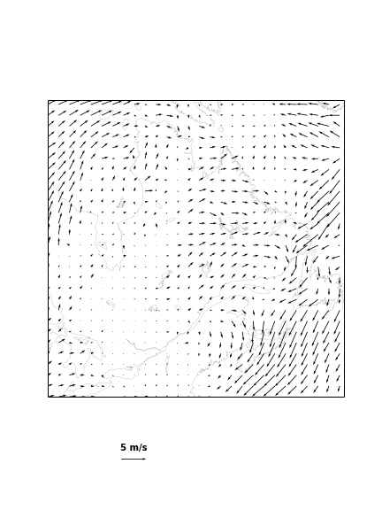
Basemap: plotting wind field (read and convert units)
download_link("http://scaweb.sca.uqam.ca/~huziy/example_data/wind.nc", "wind.nc")
ds_wind = Dataset("wind.nc")
u = ds_wind.variables["UU"][:]
v = ds_wind.variables["VV"][:]
coef_wind = 0.51444444444 #m/s in one knot
ds_wind.close()
Basemap: plotting wind field
from matplotlib.font_manager import FontProperties
fig = plt.figure()
fig.set_size_inches(6,8)
Q = b.quiver(x[::8, ::8], y[::8, ::8],
             u[::8, ::8] * coef_wind, v[::8, ::8] * coef_wind)
# make quiver key.
qk = plt.quiverkey(Q, 0.35, 0.1, 5, '5 m/s', labelpos='N',
                   coordinates = "figure",
                   fontproperties = dict(weight="bold"))
b.drawcoastlines(linewidth = 0.1);
plt.savefig("wind.jpeg");

Basemap: plotting wind field (saved image looks better)
Exercises: Basemap
Exercises: Basemap (optional)
- In the model configuration files rotated lat/lon projection is defined using coordinates of the 2 points on a rotated equator so in order to calculate parameters needed for
basemapI use this class. The methods of interest areget_north_pole_coordsandget_true_pole_coords_in_rotated_system. Try to show model domain using the following information from the model configuration file:
  4   Grd_ni        =   260  ,   Grd_nj          =   260   ,
  5   Grd_dx        =    0.1,   Grd_dy          =    0.1 ,
  6   Grd_iref      =   142  ,   Grd_jref        =   122   ,
  7   Grd_latr      =    0.0,   Grd_lonr        =  180.0 ,
  8   Grd_xlat1     =   52,   Grd_xlon1       =  -68,
  9   Grd_xlat2     =    0. ,   Grd_xlon2       =   16.65,
cKDTree
Is a class defined in
scipy.spatialpackage.Alternatives:
pyresampleandbasemap.interp
cKDTree - my workflow
1. Convert all lat/lon coordinates to Cartesian coordinates
    (xs, ys, zs) #correspond to coordinates of the source grid
    (xt, yt, zt) #coordinates of the target grid
    #All x,y,z - are flattened 1d arrays
2. Create a cKDTree object representing source grid
tree = cKDTree(data = zip(xs, ys, zs))
cKDTree - my workflow
3. Query indices of the nearest target cells and distances to the corresponding source cells
    dists, inds = tree.query(zip(xt, yt, zt), k = 1)
    #k = 1, means find 1 nearest point
4. Get interpolated data (and reshape it to 2D)
data_target = data_source[inds].reshape(lon_target.shape)
cKDTree
For an example usage of
cKDTree, please read my post at earthpy.orgThere is a folowup to that post about
pyresamplehere.
cKDTree: exercise
Interpolate CRU temperatures to the model grid, use inverse distance weighting for intepolation from 20 nearest points.
\[ T_t = \frac{\sum_{i=1}^{20}w_i T_{s,i}}{\sum_{i=1}^{20}w_i} \]
where \(w_i = 1/d_i^2\), \(d_i\) - is the distance between corresponding source and target grid points. Grid longitudes and latitudes are defined in this file. The observation temperature field is here.
Speeding up your code
Avoid loops and try to make use of Numpy/Scipy/Pandas functionality as much as possible
If you have a lot of computations the speedup can be achieved by delegating the computations to the NumExpr module.
You can use Cython to compile libraries to get C-like speed.
Use multiprocessing module if the tasks are fairly independent and cannot be solved using the above methods
Multiprocessing example
from multiprocessing import Pool

def func(x):
    return x ** 2

p1 = Pool(processes=1)
p2 = Pool(processes=2)

nums = np.arange(100000)
Make sure it works correctly
print p2.map(func, nums)[:10]
Tests of performance gain by using 2 processes instead of 1
%%timeit
p1.map(func, nums)
%%timeit
p2.map(func, nums)
Squaring example using Numpy
%%timeit
sq = np.asarray(nums) ** 2
Squaring example using NumExpr
import numexpr as ne
print ne.detect_number_of_cores()
print ne.evaluate("nums ** 2")[:5]
%%timeit
ne.evaluate("nums ** 2")
Squaring example using cythonized function
%load_ext cythonmagic
%%cython
def square_list(the_list):
    result = []
    cdef int i
    for i in the_list:
        result.append(i ** 2)
    return result
%%timeit
square_list(nums)
Resources
NumPy: http://www.numpy.org/ - there is a page NumPy for MATLAB users, might be useful for those familiar with MATLAB.
Scientific python lectures: http://scipy-lectures.github.io/
Resources
NetCDF4: http://netcdf4-python.googlecode.com/svn/trunk/docs/netCDF4-module.html
My favourite python IDE: Pycharm, you might also checkout many other like Eclipse, Netbeans, Spyder...
On creating presentations using IPython and a lot of other things: Damian Avilla's blog.